How long does SARS-CoV-2 survive outside the body?

It may not be obvious that there is a connection between the air-conditioning units of Boeing airliners, and the survival of viruses, but there is. In the 1960s, an engineer called Proschan, while working for Boeing, was studying the failure statistics of the air-conditioning units in airliners. He was a pioneer of what is often called survival analysis – the branch of statistics that deals with failure/death. The same statistics applies both to failure of a machine, or death of an organism — and to the demise of a virus, which is perhaps somewhere between a machine and an organism.

The standard, and simplest, model for survival assumes two things. The first is a constant failure/death rate, and the second is that for all the machines/living organisms, this rate is the same. Then the fraction of air-conditioning units, infectious virus etc decays exponentially

% remaining = 100*exp(-kt)

for k the failure/death rate.

Unfortunately, both these assumptions are usually wrong, even air-conditiong units are more complex than this, and living organisms are much more complex than this simple model admits. Proschan considered the case when the failure rate of each individual machine (air conditioning unit in that case) is constant, but varies from one unit to another. Then he showed that the % remaining decays more slowly than exponential. Data is then often fit with what is called a Weibull function

% remaining = 100*exp(-k’t^β)

When the exponent β < 1 the % remaining decays more slowly than exponentially.

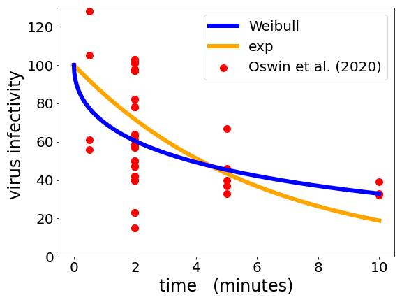
This is shown in the plot at the top of the post. The red circles are data from Oswin and coworkers on the survival of mouse hepatitis virus (MHV), a surrogate coronavirus for the other coronavirus: SARS-CoV-2. This is in aerosol droplets – which is how COVID-19 is transmitted. The blue curve is a fit of a Weibull function, with a best-fit value of β = 0.49. This is a very different function from an exponential – the bestfit exponential is shown as the orange curve.

The Weibull fit implies that as time goes on the average rage at which viruses cease to become infectious becomes slower and slower. This matters. Exponentials decay fast, for exponential decay, there is a well-defined lifetime and after about ten lifetimes then there is none left. But for the much slower decay of the blue curve above, there is no well defined lifetime. And at long times, there is much more left than with the exponential. Note that the exponential fit underestimates the data at the longest time (10 minutes). So if you want to know, for example, how long you need to wait for 99% of the virus to be no longer infectious, then it really matters which of a Weibull or an exponential is the better model.