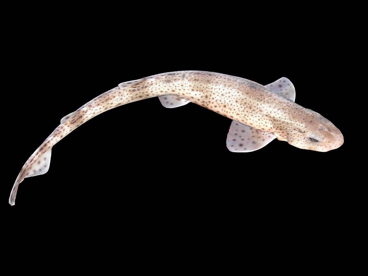
This beautiful image is of the small-spotted catshark, and is by Hans Hillewaert (Wikimedia). They are carnivores and hunt on the seabed, where I think vision is poor. So they have evolved to hunt, in part, by sensing the electric fields due to their prey. This was shown over 50 years ago, with some beautiful work by AJ Kalmijn. There is a lovely Scientific American article on this, by RD Fields, in 2007.
Author Archives: Richard Sear
Computational physicist at the University of Surrey. My research interests are in COVID-19 transmission, especially masks, soft matter & biological physics
The difference between insanity and genius is measured only by success and failure
The title is a quote by the manga artist Masashi Kishimoto. It is one of many quotes linking insanity and genius, one of them dating all the way back to Aristotle. But now, finally, we can quantify how similar insanity and madness, it is: 0.5810. This may not look that high but insanity is closer to madness than sanity, sanity and madness only have a similarity of 0.4114.
Apps for understanding better the air we breathe
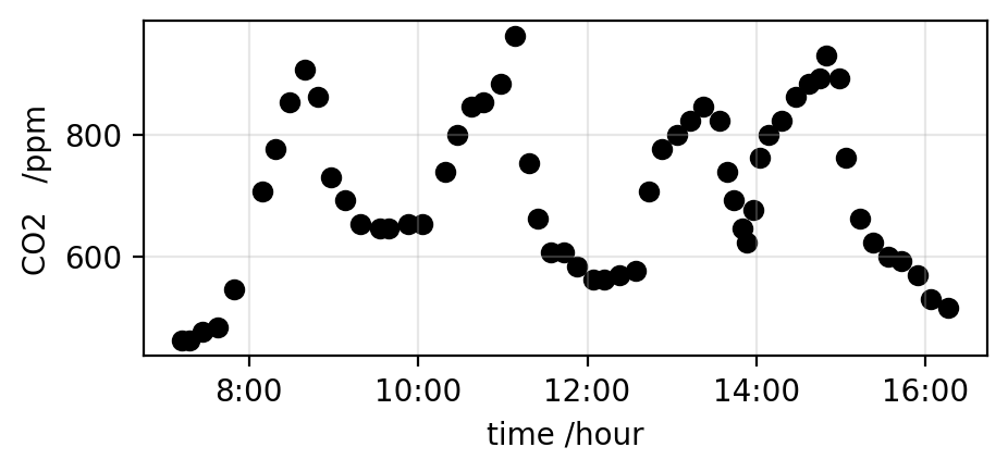
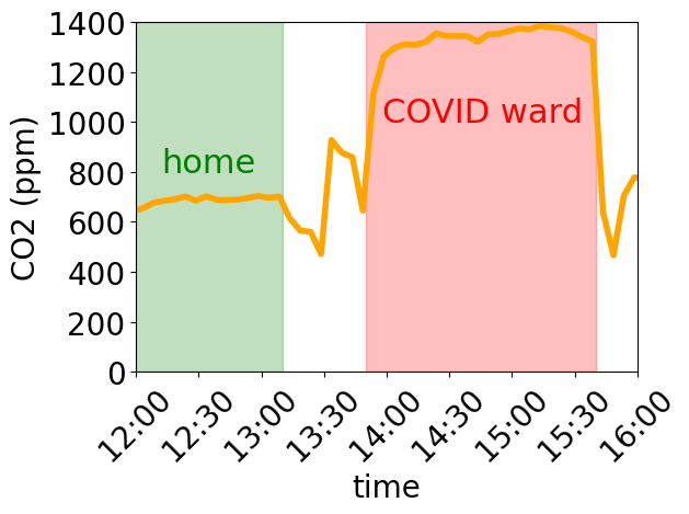
I have been suckered* into running a schools event next week, so spent most of the day writing an app to allow school kids to plot the CO2 concentration of indoor air, and do some very basic analysis. The app is now running, both on Streamlit Community Cloud and Railway*. It takes csv files that have some fraction of a day’s data on CO2 concentration in the air, and plots the data. A plot from the app is shown above. The data on CO2 levels is from a Canadian school, I thought some data on a school might be good to interest the school children.
Rattlesnakes and detecting warmth a thousandth of a degree at a time

This* is the head of a western diamond rattlesnake, a species of pit viper that is common in the USA and Mexico. Pit vipers are a family of species of snakes that called pit vipers because they have a specialised sensor organ – a pit – to detect thermal radiation (ak infrared or IR radiation). This in addition of course to their eyes which detect visible radiation. If you look carefully you can see a pit in the picture above. From left to right it lies about halfway across between the eye and the nostril, and it is close to the bottom of the head. It is hard to see because it is a pit so you really just see the shadow.
Some are born geometers, some achieve competence at geometry, and some have geometry thrust upon them
When fluids, such as air and water, flow slowly and in small systems, the equations that govern the flow simplify and become the Stokes equations. These are linear and so in simple geometries can be solved analytically, with pencil and paper. And so even before the advent of computers, a number of solutions were obtained. One of them was for flow through a circular hole in a (thin) plate. This was solved in 1891 by one Ralph Allen Sampson. The paper is a bit of a horror story of fancy maths* (in it he did many other things other than the flow through the hole) but unless I am mistaken* his result for the flow through the hole was amazingly elegant and simple, at least when viewed the right way.
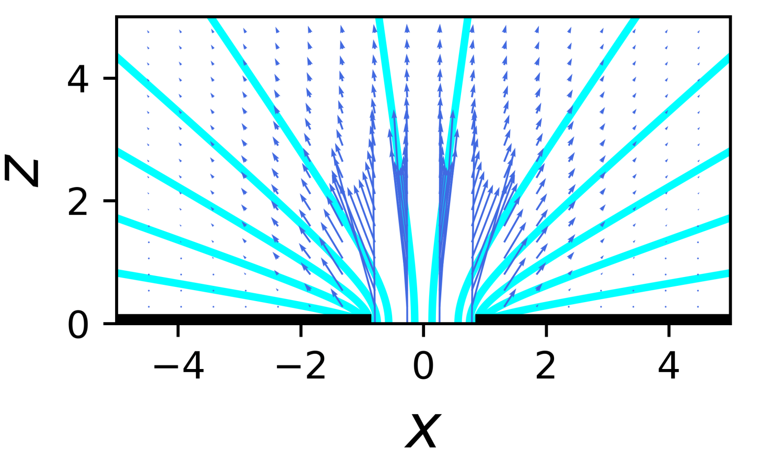
Pushing on fluids at points far from, and very near, walls
This is just a post on me teaching myself a bit about the flow patterns that occur when you apply a small force at a point in a fluid. Small here means that the flows are sufficiently small and slow that the flow is Stokes flow, i.e., the Reynolds number is close to 0.
I used LLMs a fait bit, mainly MS Copilot. The LLMs helped with elements of the problem I am interested in, but could not do the whole thing. The code to work through the flow patterns is on GitHub if you’re interested. In that sense LLMs are – very roughly speaking! – currently at the level of say a final year undergraduate lecture course on Stokes flow, but no higher. Perhaps because their training sets contains a few fluid mechanics textbooks but not enough examples beyond that. To be fair on Copilot etc clear descriptions of the problem are hard to find in the literature …
Surely microplastics are a very small problem?
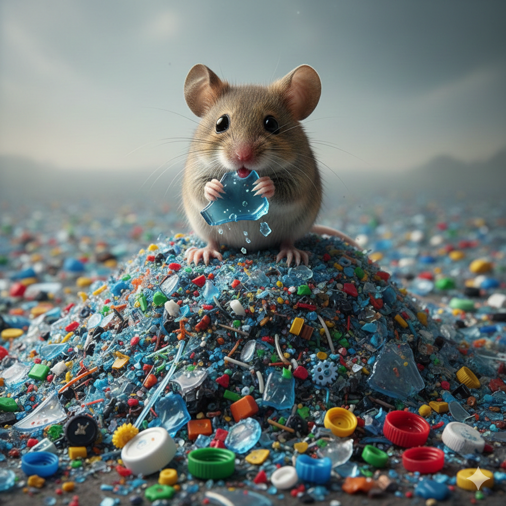
I quite like Wired magazine but it has run an article called: People Who Drink Bottled Water on a Daily Basis Ingest 90,000 More Microplastic Particles Each Year. I just cannot make sense of this. In particular I think the number 90,000 is supposed to be scarily big. But 90,000 particles of this size in one year is an absolutely tiny amount. Let me try and put the figure of 90,000 in context.
A toy app to calculate Stokes-Einstein diffusion constants
The one formula that I use above all others in my research is that for the diffusion constant of a dilute species in a fluid, called the Stokes-Einstein (or sometimes Stokes-Einstein-Sutherland) equation:
DSE = kT/(6 π η RH)
The diffusion constant DSE of something with a size (hydrodynamic radius) RH is just the thermal energy kT divided by 6π times the product of the viscosity of the fluid, η, and the hydrodynamic radius, RH. All it tells you is that large species in viscous fluids diffuse more slowly than small species in less viscous fluids.
Jumping on the LLM bandwagon with a RAGbot to answer questions on my lecture notes
Unless you have just emerged from a cave you will have heard of ChatGPT, Google Gemini, Claude, etc – collectively LLMs (Large Language Models, also called Generative AI models). Wikipedia calls Google Gemini a generative artificial intelligence chatbot. They are fancy and powerful, and touching many parts of the world including education. My employer (as I am sure many universities are) is trying to keep up.
Poor ventilation in a COVID isolation ward of NHS Wales
My mother is in a COVID isolation ward in Morriston Hospital in South Wales. COVID really knocked her out but she was mostly back to normal when I visited on Sunday (26th Oct 2025), which is a relief. The air quality in a room specifically set aside for patients infected with an disease that spreads across the air, is however pretty depressing.
