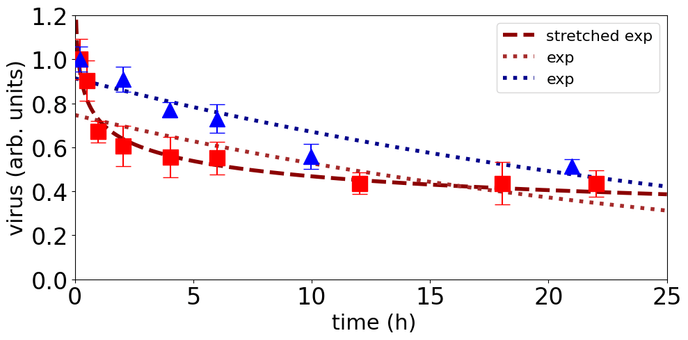
When fitting data, as in life, identifying a problem is often much easier than fixing it. There is a lot of bad fitting of data out there, and criticising it is easy. Doing a better is harder. Above are 2 sets of data on the decay of phage virus (triangles and squares) at two different temperatures. Data from work of Mathias et al. in 1995*. As the hours pass the amount of virus is reducing. We want to fit functions to the data to quantify this decrease.
The blue-triangles data is fit by a simple exponential** – the dotted blue curve. By eye the fit looks moderately bad, so easy to criticise. But how bad it is? One way to assess this is the jackknife***: a simple algorithm to test fits (models). We have 6 blue points, and dotted line is fit to all 6. But what if we leave 1 of the 6 out, fit on the remaining 5, and then see how good the fit to the 5 is at predicting the point we left out. Doing this for each of the 6 points in turn is the jackknife.
Jackknife gives an estimate of 0.13 for the root-mean-square error in the amount of virus predicted. So we estimate that within the time range we have data for (from 0 to 20 hours), our predictions from the fit will be about 13% out. This is not great, but not terrible.
What else can we predict? Once we have fit an exponential, then this immediately gives an estimate for the mean lifetime for the virus, and with a jackknife estimate of the uncertainty we get a mean virus lifetime of 32 h, with an uncertainty of 7 h.
We have also fit an exponential (red dotted curve) to the red square data. This is also for virus survival but at a different temperature. That fit looks a pretty terrible fit by eye, although the jackknife estimate of prediction error in the time range studied, is 0.15, only 0.02 larger than for the blue data.
Can we do better with another function? We can try a stretched exponential:
In comparison to the exponential, this has an parameter, the exponent β, in addition to the timescale τ and the initial amount of virus I0. When the exponent β = 1 we get back the exponential we tried first, but when the exponent is < 1 then we get an initial rapid decrease, which then slows, which is what the red data does.
The stretched exponential is the dark-red dot dashed curve, and indeed the jackknife error of the prediction error is indeed smaller. It is halved at 0.07 versus the exponential’s 0.15. So it looks better at estimating the fraction of virus remaining, within the time range we have data for. By that criterion we have improved the fit.
So we have what looks like a reliable way of predicting the remaining fraction of virus, over the period studied, from 0 to 20 hours. What about the predicted lifetime?
For the exponential we have a predicted lifetime of 29 h, with an uncertainty of 4 h. And for the stretched exponential a predicted lifetime of 6500 years (not hours)! To put it mildly, our estimate of the virus lifetime seems very model dependent.
The decay is clearly slowing a lot, and maybe it is plateauing – i.e., a fraction of the virus does not decay in anything like the tens of hours studied. But maybe it is not. The data can’t tell, and this matters for the lifetime, but not really for the in time-range predictions of fraction left. If there is a real plateau then the lifetime is infinite.
So, it looks like with a bit of fitting we can predict the fraction of virus remaining in the time range studied, but can say essentially nothing about the virus’s lifetime. The data don’t allow lifetime estimation. A better fit function cannot fix that, although comparing predictions from different functions can show the problem. But a better function can improve in-time-range predictions.
* Mathias and coworkers were interested in phages – virus that infect bacteria – in the Danube. Data is from the middle panel of their figure 5. Here I am using just it as data of something decaying.
** All fits and data are in a Google Colab notebook.
*** jackknife is a form of cross validation or out of sampling testing of a model or fit. Here testing means means the ability of the fit to predict, here, the amount of virus left.


