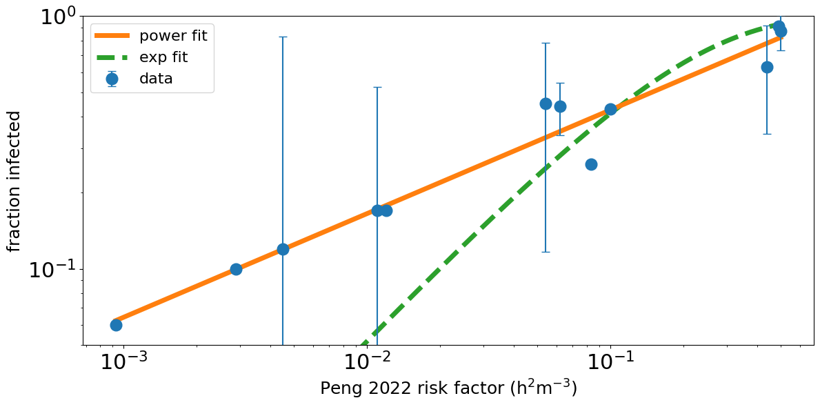
Peng and cowokers gathered together data on 12 (possibly not very representative) events where COVID was transmitted. For each event they estimated a relative infection risk factor Hr*. They then plotted the fraction of people infected (an estimate of the probability of infection), as a function of this estimated relative risk factor. They compared with the standard model for disease transmission – the Wells-Riley model (which is really just Poisson statistics). A fit of this model to their data is shown as the green dashed curve in the plot above. It is not a great fit**.
In particular the fit drops off too fast at low values of the infection risk factor. The functional form of the Wells-Riley model is
where there is one fit parameter, the scale factor for the risk factor SH. The functional form of the Wells-Riley model has built into it that the infection probability increases from small to large infection probabilities over a range of values Hr that is comparable to the scale SH. Here small is 0.1 or less and large is around 0.9 or more. For this data the best fit scale SH = 0.19, and so as the risk factor drops to values much less than SH the infection probability drops rather rapidly (linearly) while the drop in the data is much slower.
The values of the risk factors estimated by Peng and coworkers span more than two decades. When data spans multiple decades, power laws are often sensible simple models to use. Here a power law is
The solid orange line in the plot above (note plot is log-log) is a power law fit**, with exponent β=0.41. It is a much better fit than Wells-Riley.
A power law with exponent a bit less than a half matches the slow increase in infection probability, with increasing values of the exposure, as measured by the Peng and coworkers relative risk factor.
This slow power law increase of infection probability with exposure is similar to that found in data from the NHS COVID-19 app many of us used during the pandemic. Power law fits were done in the original analysis by Ferretti and coworkers***, and by me (see earlier post). For the data the best fit exponent was β = 0.48, i.e., only a little bit higher than for the fit above.
The x axis was different in that data, and in both cases power laws are very simple models of very complex phenomena. But as they are so simple, perhaps they are useful, and they often seem much better fits than the conventional Wells-Riley model**.
* The relative risk factor of Peng and coworkers is defined by
with
and rSS, rE and rB factors that account for (in order): the amount of virus in the air not having time to reach steady state; for activities (eg singing) expected to increase emission rate above that of a person at rest; activities (eg running) expected to increase breathing rate above that of a person at rest.
** The R2 = 0.79 for the Wells-Riley (Poisson stats) fit and 0.92 for the power law fit. Fits done in Google Colab notebook here. N.B. Three comments: I. Comparison between the two fits is not 100% fair as Wells-Riley only has 1 fit parameter, while the power law has 2. II. Both fits are perhaps misleadingly good as the risk factor of Peng and coworkers includes parameters they and other workers have adjusted. III. With a simple power law, the probability can exceed 1 which is obviously wrong but this can be fixed by going over to a stretched exponential.
** Ferretti and coworkers seem to (partially?) disown the power law fits in their Extended Data Fig 2, by saying that at short exposures “the relationships were approximately linear …. as expected from theoretical arguments”. But they don’t specify what these “theoretical arguments” are, so I am a bit confused here.


1 Comment