I am no expert but as I understand it, a lot of LLMs like Anthropic’s Claude, and image generators like Stable Diffusion, are built on neural nets. And a lot of these neural nets are trained via backpropagation. I want to understand a little more about this, and maybe teach a simple example in my Python course – although this may be a little advanced for first year physicists. So first I need to teach myself a little about both how a neural net works and backpropagation works.
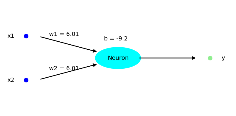
I think that if you want to understand something it is best to start with the simplest example, so my neural net – see above – is in fact just one single model neuron – as opposed to the billions of artificial neurons (arranged in many layers) in the AI tools we use. I think a neural net is basically just a flexible trainable function. In other words it is a function, i.e., you put in one or more numbers (in my example two numbers), and get out another number. And it is trainable in the sense that the neural net has parameters (3 in my case, billions plus in the case of the ones in LLMs etc) whose values can be varied to allow the function to do almost anything, to mimic almost any function you want (eg “denoise” an image, see earlier post).
The function part of my neuron is easy, the function’s
while the
and the function has
As there are only three we can’t train the neural net (single neuron) to be a fancy function but we can train it to be a simple function: the AND gate.
To do this we need the training data, which are the 4 correct input/output pairs for an AND gate:
So 4 input/output pairs defines the simple function that is an AND gate. It is this function we want our toy neural net to mimic.
To do this we need to work out what values for the weights and bias parameters give a function closest to the AND-gate function. This is where backpropagation comes in, but first we need to define a loss or error function to quantify how bad/good the neuron is at mimicking the AND-gate function. We go for
where
and we sum (using α) over the n = 4 input/output pairs in the training.
This loss function L is zero when each of the four predictions is perfect and increases, the worse these predictions are. This is just one choice of loss function, there others with the same property.
The backpropagation method for training starts with a loss function, then needs the derivative of this loss function with respect to the parameters, eg with respect to a weight
This result is obtained after quite a lot of chain rule differentiation. Given how important backpropagation is to modern AI, this must be at least the most topical reason to learn chain rule calculus. The explicit chain-rule differentiation is in a Google Colab notebook, which also runs the neuron and did the plot up top.
One comment: The magic of backpropagation is that it is efficient for neural nets of many layers (as the big commercial ones underlying Google Gemini all are). This does not come across as my net is so simple there is only one layer.
The above equation for the derivative basically says that the rate of change of the loss function with respect to a parameter (weight) is minus the average error in the output prediction (term in []) times the input with that weight. Note that this means that when the prediction is perfect, the derivative is zero. When the prediction is too high, then the derivative is positive, while if the prediction is too low, the derivative is negative.
This means we can use the derivative to both say which direction we should change the weight’s value to make the neuron better mimic – the opposite of the sign of the derivative – and to guesstimate how big a change we should make. It should be large if the derivative is large as then it looks like we can greatly improve the function, small if the derivative is small as there we may be need the optimum value (where derivative is zero).
In practice backpropagation then starts off with a guess for each parameter value, then iteratively updates each parameter, according to the rule
where ρ is a learning rate parameter. If the predictions are, on average, too high then the weight is reduced by an amount proportional to how fast the loss function varies with that weight, and modulated by a learning rate parameter. This is basically just an example of the standard optimisation method of gradient descent.
Then after a 100 or 1000 iterations, hopefully the neural net mimics the function you are training on, here the AND gate. After 100 iterations, my code gives the weight values given in the image above. And the now trained neuron gives:
which is pretty close to the correct table above. With a bias of −9.2 when the inputs are 0 then the output is very close to 0 – see the output function above. As the bias is larger in magnitude than each weight individually (9.2>6.01) then if only one input is 1 then the output is still quite small. But when both inputs are one the output is close to one, as the magnitude of the bias is less than twice the value of each weight.
So the neuron works as a good mimic of the AND gate. As my example is so simple the advantages of backpropagation cannot really be seen – that would require multiple layers and a much more complex problem. But it still shows some of the ideas that are currently changing our world.
