Pushing on fluids at points far from, and very near, walls

This is just a post on me teaching myself a bit about the flow patterns that occur when you apply a small force at a point in a fluid. Small here means that the flows are sufficiently small and slow that the flow is Stokes flow, i.e., the Reynolds number is close to 0.

I used LLMs a fait bit, mainly MS Copilot. The LLMs helped with elements of the problem I am interested in, but could not do the whole thing. The code to work through the flow patterns is on GitHub if you’re interested. In that sense LLMs are – very roughly speaking! – currently at the level of say a final year undergraduate lecture course on Stokes flow, but no higher. Perhaps because their training sets contains a few fluid mechanics textbooks but not enough examples beyond that. To be fair on Copilot etc clear descriptions of the problem are hard to find in the literature …

Let us start easy: in the Stokes (small and slow flows) regime the effect of a force exerted at a point in a fluid far from any boundary, creates what is called Stokeslet flow. A Stokeslet flow of strength F parallel to the z axis in free space, is the flow velocity field:

this is in Cartesian coordinates, and in the y = 0 plane, so the y component is zero. Out of this plane there is a y component that is analogous to the x component (as the applied force is perpendicular to both the x and y axes). The Python/Sympy/Pyplot code for all the maths and plots is in a Jupyter notebook on GitHub.

Flows can be visualised by means of streamline plots: plots of curves that follow the trajectories of packets of fluids or particles if these particles are being carried by the flow. The curves have arrows to indicate the direction of travel. The streamline plot (in 2D, the xz plane) for a Stokeslet in the bulk of a fluid is:

In the bulk, if you push with a force at the point then this pushes the surrounding fluid into motion along the direction of the force. As you can see the motion also tends to pull the fluid behind the point where the force is exerted (red disc), in towards it. This gives a ‘waist’ to the streamlines, but the predominant direction is forward, and the flow is relatively uniform.

The math expression above tells us that the effect of the applied force on the fluid is very long range, the flow velocity only decays as 1/r, where r is the distance from the force*, i.e., if you double the distance from the point where the force is exerted, the velocity only halves (as opposed to say exponential decay which would be much faster). If you push on a point in the bulk of the fluid, then you push a large volume of the fluid into motion.

As has been appreciated, since the 19th century I think, the situation when a force is applied at a point near a surface, is very different. If the force is applied, for example, perpendicular to and pointed away from a wall, then it can’t pull much fluid from behind it, as the wall is in the way.

And typically, in a fluid as a wall is approached the velocity along the wall also tends to zero: the fluid immediately in contact with the wall cannot move as it stuck to the wall by friction. So along the wall all components of the flow velocity are zero. This limits the flow induced by pushing at a point just above this wall.

So when we exert a force close to a wall we want a solution of the relevant equations (Stokes’ equation) that looks like the Stokeslet in the bulk very close to the point (much closer than h if h is the distance between the wall and the force) and that satisfies the zero flow condition at the wall. This is done by using the fact that Stokes’ equation are linear and homogeneous so the sum of any solutions is itself a solution. So what is done is add enough solutions to the bulk Stokeslet to satisfy this condition at the wall.

This I understand. What I do not understand – it looks like magic to me although it is maths not magic – is what these solutions are. In fact as Blake and Chwang showed in the 1970s, the flow field from Stokeslet of strength F, h above and perpendicular to a wall, is the sum of 4 flow fields. These 4 are:

1. flow field of free space Stokeslet of strength F h above the wall
2. flow field of free space Stokeslet of strength −F −h below the wall
3. free space “Stokes doublet” of strength (2Fh) −h below the wall
4. free space “source dipole” of strength (Fh²) −h below the wall

If you add these 4 together you get the flow field:

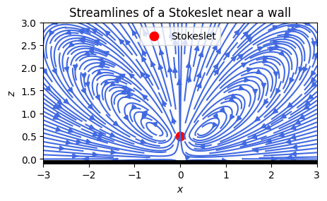
which is quite pretty. Note that the large lateral flows near the wall (wall is shown in black) needed to pull in fluid to be pushed up by the force. This creates distinctive ‘bunny ears’ vortex like flow patterns. The full flow field is three dimensional, the above is just a slice through it, so the ‘bunny ears’ are slices through a roughly oval, donut-shaped vortex that rings and is just above the point where the force is applied.

The flow tends to zero as h -> 0, as the stick boundary conditions at the wall suppress flow. So the flow pattern can be written as an expansion in h, with the h = 0 term equal to 0. In fact for reasons I don’t really follow the linear term in h is also 0. And so the leading term is the h² term, which is:

Note that it scales as 1/r³, i.e., it decays much faster than in the bulk. In the bulk if you double the distance to the force, the flow velocity halves, here it drops by a factor of 8. Also note that every term has a factor of z in it, and so the flow velocity equals 0 when z = 0. This mean it satisfies the boundary conditions at the wall**.

A plot of this single term is:

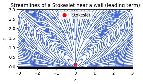
which is pretty similar to the plot just above of the full flow velocity field. There are only small differences near the Stokeslet (red disc), while it is almost identical far from the Stokeslet. This is as it should be. It is longest range term, which should be better at larger distances from the point where the force is applied.

So, with some help from LLMs, but using Blake and Chwang’s paper is the reference, I now have a better understanding of the, fascinating I think, problem of flows near walls.

* The 1/r dependence is clear from the last term but all terms, e.g., xz/r_³ have the same 1/r scaling.

** The streamlines near the wall (in black) are close to horizontal, presumably because the tangential component of the velocity scales as z, while the normal component scales as z² – a much faster decrease as the wall is approached.