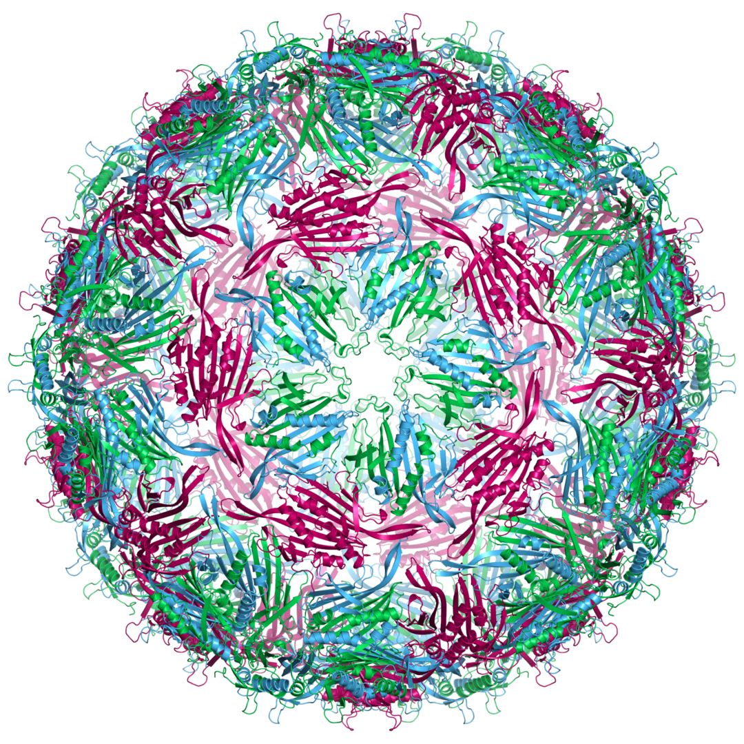
Above is avery pretty cartoon/schematic* of a virus MS2 that infects bacteria. I think it is used in proof-of-principle studies with viruses, as it is safer/easier/cheaper to work with than viruses that infect us. The virus can become airborne, which brings us to air conditioning units, which typically have filters as part of them. The filters can filter out viruses such as MS2 from the air.
Back in the early 1960s, an engineer called Proschan studied data on breakdown statistics of air conditioning units of early airliners. Now the most basic model for these statistics is that each unit fails at some constant fixed rate (i.e., probability per flight), and then the fraction still working after a given time decays exponentially with that time. Proschan realised that if indeed each unit had a constant failure rate, but that the units were heterogeneous in the sense that this rate varied from one unit to another, then the fraction still working would always decay more slowly than exponentially.
The argument for this is pretty trivial. At early times units with both large and small failure rates are present, but the decrease in the fraction of units still working is fast as it is driven mainly by the failure of the units with intrinsically high failure rates. Then at later times, most of the units with high failure rates have already failed so the average failure rate is now much lower, as only units with low failure rates are left.
This takes us back to the virus MS2, and some very nice recent work by Ratliff and coworkers. They studied the fraction of viable MS2 left in an aerosol (i.e., airborne small particles), as a function of time. The droplets are the virus immersed in a model of our saliva. Viruses are fragile and can’t reproduce outside of a host so the fraction left decays as the viral particles are destroyed and not replaced. Ratliff et al.’s data is below as the points:
The black points are just for MS2 decaying in the aerosol, while the red points are when the aerosol is exposed to UVC light which can damage the virus, and the blue points are with an air filter (HEPA) that can filter out the virus-containing aerosol.
The dashed cyan curves are fits to the data of exponential decays. And as the y axis is a logscale, this curves are straight lines on this plot. They are not great fits. In particular in all three cases the exponential fits underestimate the final value, just what you would expect if the overall rate of decrease is slowing. And the overall rate will decay if in some fraction of the aerosol droplets the virus was decaying faster than in other droplets.
At the cost of a second fit parameter, the fit can be improved. The orange curves are fits of stretched exponentials aka Weibull functions, exp[-(t/t*)β], with β an exponent < 1, and t* a timescale. For the fits above β is around 0.6 to 0.75, which gives a modest amount of slow down in the decay rate (when β = 1 we are back to simple exponential decay).
These values of β also correspond to an apparent modest heterogeneity in the decay rate of the virus, under all three conditions, with and without UVC light and filtration. This is I think quite a complex problem so there are many possible sources of the heterogeneity. There could be heterogeneity in the virus and model-saliva droplets. The air in different parts of Ratliff et al.‘s system may mix a different rates and this may introduce heterogeneity into the studies with UVC and filtration, etc.
A slower-than-exponential decay of the virus means that at least a small amount of virus survives for long times. It also makes it harder to estimate the amount of virus left after long times, if you only have data at shorter times, and the standard model for airborne transmission of viral diseases – the Wells-Riley model – assumes exponential decay. For all these reasons, it is good to know the functional form of the decay.
*Cartoon of the virus MS2 is by Naranson – and is CC BY-SA 3.0
