Power laws and COVID

Above is a plot of the data of Ferretti and coworkers (green circles and crosses*) on the probability of infection with COVID, as a function of exposure, as measured by data from the NHS COVID-19 app. Note that it is on a log-log scale. The blue line is a power-law fit*, with best fit exponent β = 0.48, i.e., the probability of infection almost scales as the square root of the exposure (that would be β = 1/2). For comparison there is also a line (orange) showing what linear behaviour (β = 1) would look like. Clearly the data look a long way away from linear. And indeed Ferretti and coworkers do fit power laws and also get good fits, and a similar exponent.

I would say that the power-law fit is pretty good. Power laws only have two parameters so this is a simple empirical model, that can economically summarise the data. But is it anything more?

Maybe it is. Power laws very often occur when there is a broad distribution of things. A classic example is earthquakes, whose energies vary from barely enough to rattle some crockery to enough to level large buildings – this is a huge range. The distribution of earthquake energies is approximately a power law. But the viral load of people infected with COVID also known to span a huge range.

If** this translates into a huge range of infectiousness, then the rate of transmission r may vary over a huge range. Essentially, one susceptible person may be sharing a room with someone breathing out lots of virus and so be infected after minutes, while another may be sharing a room with an infected person breathing out orders of magnitude less virus. Then it may take hours or days in the same room or house to become infected, or they may not become infected at all. This implies** a broad distribution of infection rates, from one encounter to another. The probability distribution function for the transmission rates p(r) may then be a power law, i.e., p(r) ~ r^-x with x the exponent of the power law.

Then a simple model for the probability of being infected after a time t, is that the probability of becoming infected is just the fraction of encounters where the transmission rate was high enough to infect within the time t ~ 1 / r. Then the probability of becoming infected after a time t is

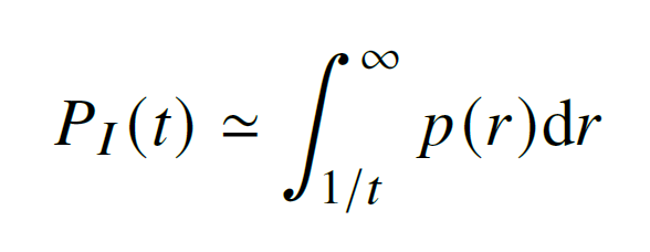
Now if p(r) ~ r^-x with say x = 3/2, then on doing the above integral we get a P_I(r) ~ t^1/2. This is pretty much what Ferretti and coworkers see.

So if indeed there is huge range in the rate at which the virus is transmitted, from one encounter of a susceptible person with an infected person, to another, then a power law is very likely. And this has consequences. If the infection probability is linear, then say doubling the ventilation halves the infection probability. But it is isn’t, so doubling the ventilation probably only reduces the infection probability by about 30%.

* Fit is of a straight line to the log of the infection probability as a function of the log of the app-estimated risk. Only the first 12 of the 15 data points are used for fitting. These 12 are circles, other 3 are crosses. For the fit R² = 0.99. The log residuals looks like:

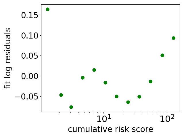
This is clearly not random noise, there is a small amount of wiggling about the fit. I don’t know what this is. Fitting is with Python’s scipy’s linregress which gives a standard error on the exponent of 0.015, so true exponent could be 1/2 but is absolutely not 1.

** This is quite a big if.