Teaching elementary machine learning

Next semester I will be teaching a computational modelling course, to second-year physics undergraduates. The projects are mainly standard computational physics projects, like computing the orbits of the planets. Currently there is no machine learning (ML) project. Given how topical ML is, and how many jobs there in ML, this is perhaps a bit of an omission. I am working on fixing this, by developing a simple supervised learning ML project: Predicting probabilities of developing heart diseases using logistic regression.

The data is from the Framingham (Massachusetts, USA) heart study, a study of heart disease that has been ongoing in Massachusetts since 1948. I downloaded a dataset of Framingham data, of Ashish Bhardwaj on Kaggle, and the analysis in this post is heavily inspired by (the first half of) a Jupyter notebook of Nisha Choondassery, also on Kaggle.

Logistic regression is where we fit the logistic function p(x):

p(x) = 1 / [ 1 + exp( −β₀ −β₁x) ]

to the data. Here the probability p is of a variable x which is either 0 or 1, i.e., x is not continuous, it is a binary variable. In this case x = 1 if someone develops heart diseases within a ten-year period, and is 0 if they do not develop heart disease within ten years. The logistic function is basically the simplest function that goes continuously from 0 (at x = − ∞) to 1 (at x = ∞), and so logistic regression is basically the analog for a binary variable x, of linear regression for a continuous variable x. A straight line is basically the simplest function for a continuous variable.

The dataset from Kaggle has over three thousand surveyed people in it. For each person there are a number of potential risk factors for heart disease, plus whether in a ten-year period the person does or does not develop heart disease. One of these risk factors is age, in the range 30 to 70 years old. Above, I have binned the data in decade wide bins, and just plotted the fraction of people in each decade that go to develop heart disease – these are the blue bars.

The logistic-function fit is shown as the red curve, and the bestfit values are: β₀ = −5.7 and β₁ = 0.077. The simple functional form of the logistic function looks OK, except perhaps for overestimating how steep the increase in risk is, in the 70s. The logistic function can be rewritten as

ln [ p(x)/(1-p(x)) ] = β₀ + β₁x

Now p(x)/(1-p(x)) is just the odds ratio of getting heart disease in the ten-year period, e.g., if 1 out of 10 get heart disease while 9 out of 10 don’t, p(x)/(1-p(x)) = 1/9. So we can write this as

ln [ odds ratio of getting heart disease in ten years ] = −5.7 + 0.077 * [age in years]

So, the odds ratio starts off very small when you are young, but is predicted to increase approximately as exp(0.077 * [age in years]) as you age. The plot of the log of the odds ratio looks like:

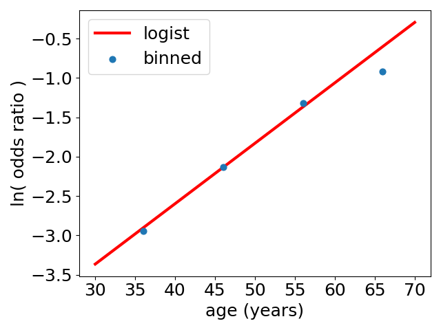
As you can see it is not very far from a straight line, apart from overpredicting the risk for people in their 70s. It looks like an exponential growth of the odds ratio for heart disease is a pretty reasonable first approximation., and so the logistic model is a sensible way of predicting how the risk of heart disease varies with age.

This is the supervised-learning flavour of ML. It is “supervised” because we give the algorithm/model (here the logistic function) data with both the variable we want to use as input to make predictions with (the age), and what we want to predict (heart disease), it is the latter that provides the “supervision”. Now that we have, in ML language, trained the model with the Framingham data, we can use it to make predictions, of the probability of developing heart disease.